Using flextable with ggplot2 and patchwork
Original dataviz is available at https://insights.datylon.com/stories/oDHVikVxaCaCGWRFGMdPgA.
Get the data
library(readxl)
library(tidyverse)
library(magick)
## Linking to ImageMagick 6.9.12.3
## Enabled features: cairo, fontconfig, freetype, heic, lcms, pango, raw, rsvg, webp
## Disabled features: fftw, ghostscript, x11

scoring_data <- read_excel("default_workbook.xlsx",
           sheet = "Scoring data") %>%
  rename(name = NAME, pts = PTS, fgp = "FG%", group = Group) %>%
  mutate(pts = as.double(pts),
         fgp = as.double(fgp))
scoring_data
## # A tibble: 581 × 4
##    name                    fgp   pts group
##    <chr>                 <dbl> <dbl> <chr>
##  1 Joel Embiid            49.9  30.6 Ineffective high-scorer
##  2 LeBron James           52.4  30.3 Effective high-scorer
##  3 Giannis Antetokounmpo  55.3  29.9 Effective high-scorer
##  4 Kevin Durant           51.8  29.9 Effective high-scorer
##  5 Luka Doncic            45.7  28.4 Ineffective high-scorer
##  6 Trae Young             46    28.4 Ineffective high-scorer
##  7 DeMar DeRozan          50.4  27.9 Effective high-scorer
##  8 Kyrie Irving           46.9  27.4 Ineffective high-scorer
##  9 Ja Morant              49.3  27.4 Ineffective high-scorer
## 10 Nikola Jokic           58.3  27.1 Effective high-scorer
## # … with 571 more rows
For the images in the table, you have to create a data.frame manually. We will download each image in a temporary file because flextable only manages locally available images.
head_shot <- tibble::tribble(
  ~name, ~url,
  "Joel Embiid", "https://cdn.nba.com/headshots/nba/latest/1040x760/203954.png",
  "LeBron James", "https://cdn.nba.com/headshots/nba/latest/1040x760/2544.png",
  "Giannis Antetokounmpo", "https://cdn.nba.com/headshots/nba/latest/1040x760/203507.png",
  "Kevin Durant", "https://cdn.nba.com/headshots/nba/latest/1040x760/201142.png",
  "Trae Young", "https://cdn.nba.com/headshots/nba/latest/1040x760/1629027.png",
  "Luka Doncic", "https://cdn.nba.com/headshots/nba/latest/1040x760/1629029.png"
) %>%
  mutate(url = map_chr(url, function(z) {
    path <- tempfile(fileext = ".png")
    image_read(z) %>%
      image_resize(geometry = "144x") %>%
      image_write(path = path)
    path
  }))
The table ‘Q3_data’ will be used when building the ggplot.
Q3_data <- summarise(scoring_data,
          pts = quantile(pts, probs = .75),
          fgp = quantile(fgp, probs = .75)
          )
Q3_data
## # A tibble: 1 × 2
##     pts   fgp
##   <dbl> <dbl>
## 1  11.3    50
The ‘scoring_highlight’ table will be the main table.
scoring_highlight <- scoring_data %>%
  arrange(desc(pts), desc(fgp)) %>%
  slice_max(pts, n = 6) %>%
  left_join(head_shot, by = "name")
scoring_highlight
## # A tibble: 6 × 5
##   name                    fgp   pts group                   url
##   <chr>                 <dbl> <dbl> <chr>                   <chr>
## 1 Joel Embiid            49.9  30.6 Ineffective high-scorer /var/folders/08/2qd…
## 2 LeBron James           52.4  30.3 Effective high-scorer   /var/folders/08/2qd…
## 3 Giannis Antetokounmpo  55.3  29.9 Effective high-scorer   /var/folders/08/2qd…
## 4 Kevin Durant           51.8  29.9 Effective high-scorer   /var/folders/08/2qd…
## 5 Trae Young             46    28.4 Ineffective high-scorer /var/folders/08/2qd…
## 6 Luka Doncic            45.7  28.4 Ineffective high-scorer /var/folders/08/2qd…
Do the flextable
theme_scorer <- function(x) {
  border_remove(x) %>%
    valign(valign = "center", part = "all") %>%
    align(align = "center", part = "all") %>%
    fontsize(part = "all", size = 20) %>%
    bold(part = "header", bold = TRUE) %>%
    bold(part = "body", j = 1, bold = TRUE) %>%
    color(color = "#b17268", part = "header") %>%
    bg(part = "header", bg = "transparent")
}

ft <- as_grouped_data(scoring_highlight, groups = c("name"), expand_single = TRUE) %>%
  as_flextable(hide_grouplabel = TRUE, col_keys = c("url", "fgp", "pts")) %>%
  set_header_labels(url = "", fgp = "Field goal", pts = "Points") %>%
  mk_par(j = "url", i = ~ !is.na(url),
         value = as_paragraph(
           as_image(url, width = .75, height = 0.54),
           "\n",
           as_i(name)
           )
         ) %>%
  theme_scorer() %>%
  align(i = ~!is.na(name), align = "left", part = "body") %>%
  bg(i = ~ group %in% "Effective high-scorer", bg = "#f8b26399") %>%
  bg(i = ~ group %in% "Ineffective high-scorer", bg = "#b1726899") %>%
  hline(i = rep(c(FALSE, TRUE, FALSE, TRUE), length = nrow_part(.))) %>%
  autofit()
We can already see the table as a plot.
plot(ft, fit = "fixed", scaling = "fixed", just = "centre")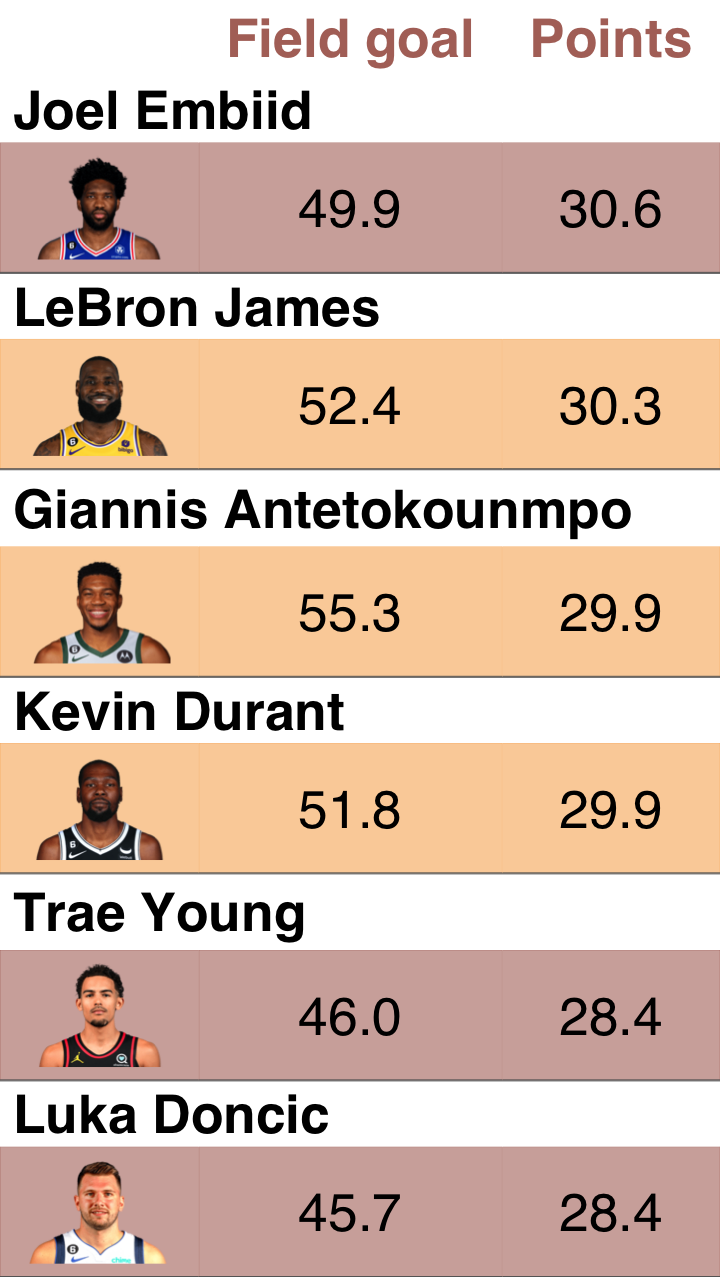
Do the ggplot
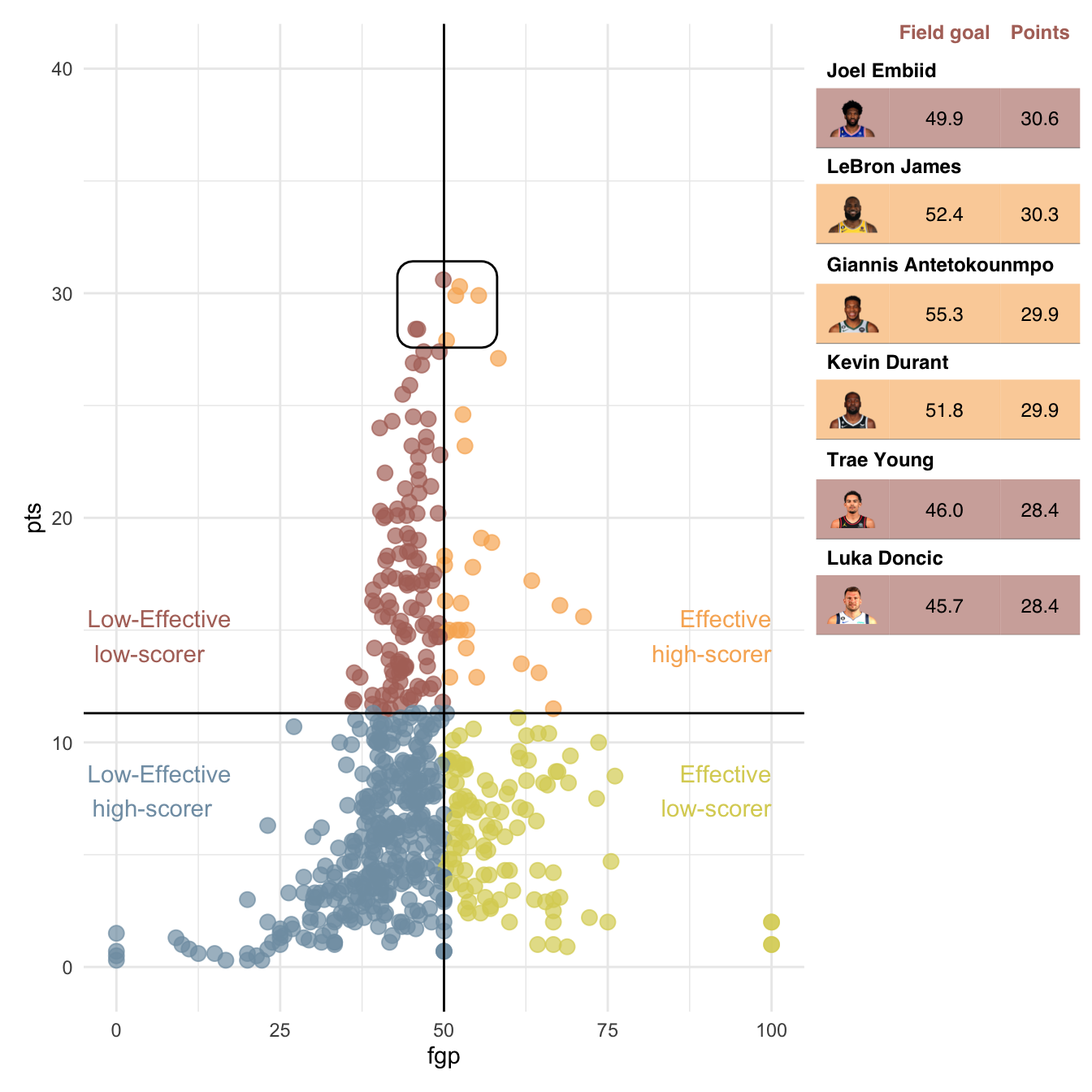
gg <- scoring_data %>%
  ggplot(mapping = aes(x = fgp, y = pts, color = group)) +
  geom_point(size = 3, alpha = .7, show.legend = FALSE) +
  scale_color_manual(
    values = c(
      "Effective high-scorer" = "#f8b263",
      "Ineffective low-scorer" = "#819eb2",
      "Ineffective high-scorer" = "#b17268",
      "Effective low-scorer" = "#dad162"
      )) +
  scale_y_continuous(limits = c(0, 40)) +
  geom_hline(data = Q3_data, aes(yintercept = `pts`)) +
  geom_vline(data = Q3_data, aes(xintercept = fgp)) +
  ggforce::geom_mark_rect(data = scoring_highlight,
                   mapping = aes(color = NULL),
                   expand = unit(3, "mm"),
                   show.legend = FALSE) +
  annotate(geom = "text", x = 100, y = Q3_data$pts,
           label = "Effective\nhigh-scorer", color = "#f8b263",
           hjust = 1, vjust = -1) +
  annotate(geom = "text", x = 100, y = Q3_data$pts,
           label = "Effective\nlow-scorer", color = "#dad162",
           hjust = 1, vjust = 2) +
  annotate(geom = "text", x = 0, y = Q3_data$pts,
           label = "Low-Effective\nhigh-scorer", color = "#819eb2",
           hjust = 0.2, vjust = 2) +
  annotate(geom = "text", x = 0, y = Q3_data$pts,
           label = "Low-Effective\nlow-scorer", color = "#b17268",
           hjust = .2, vjust = -1) +
  theme_minimal()
gg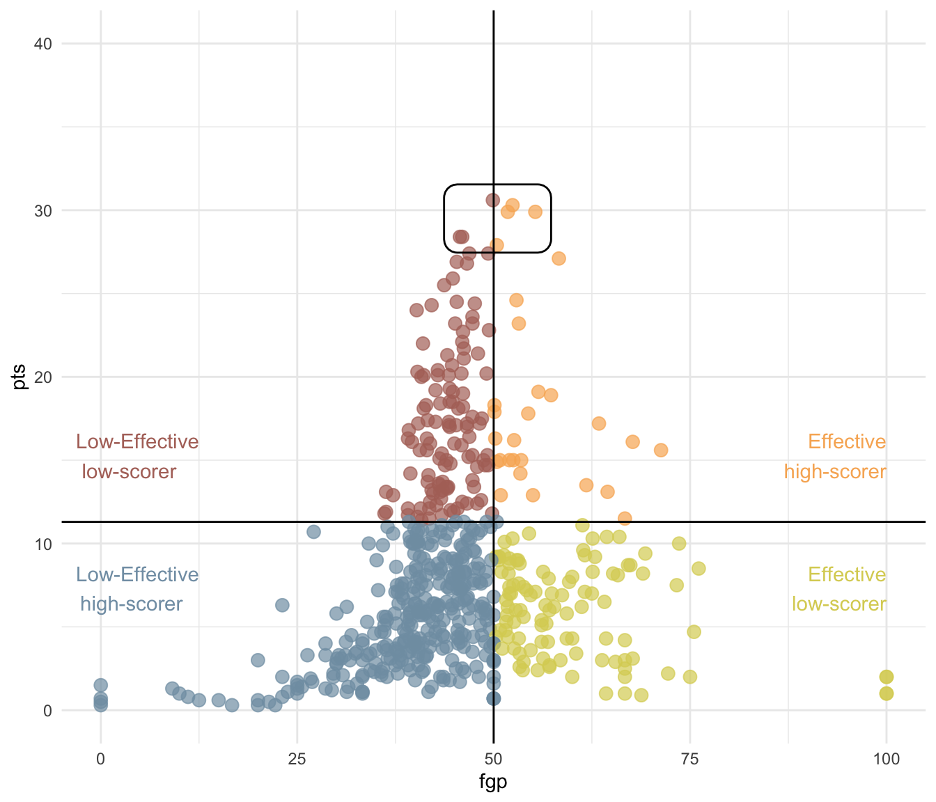
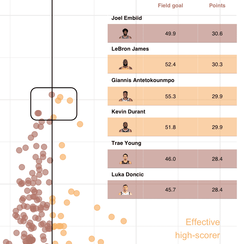
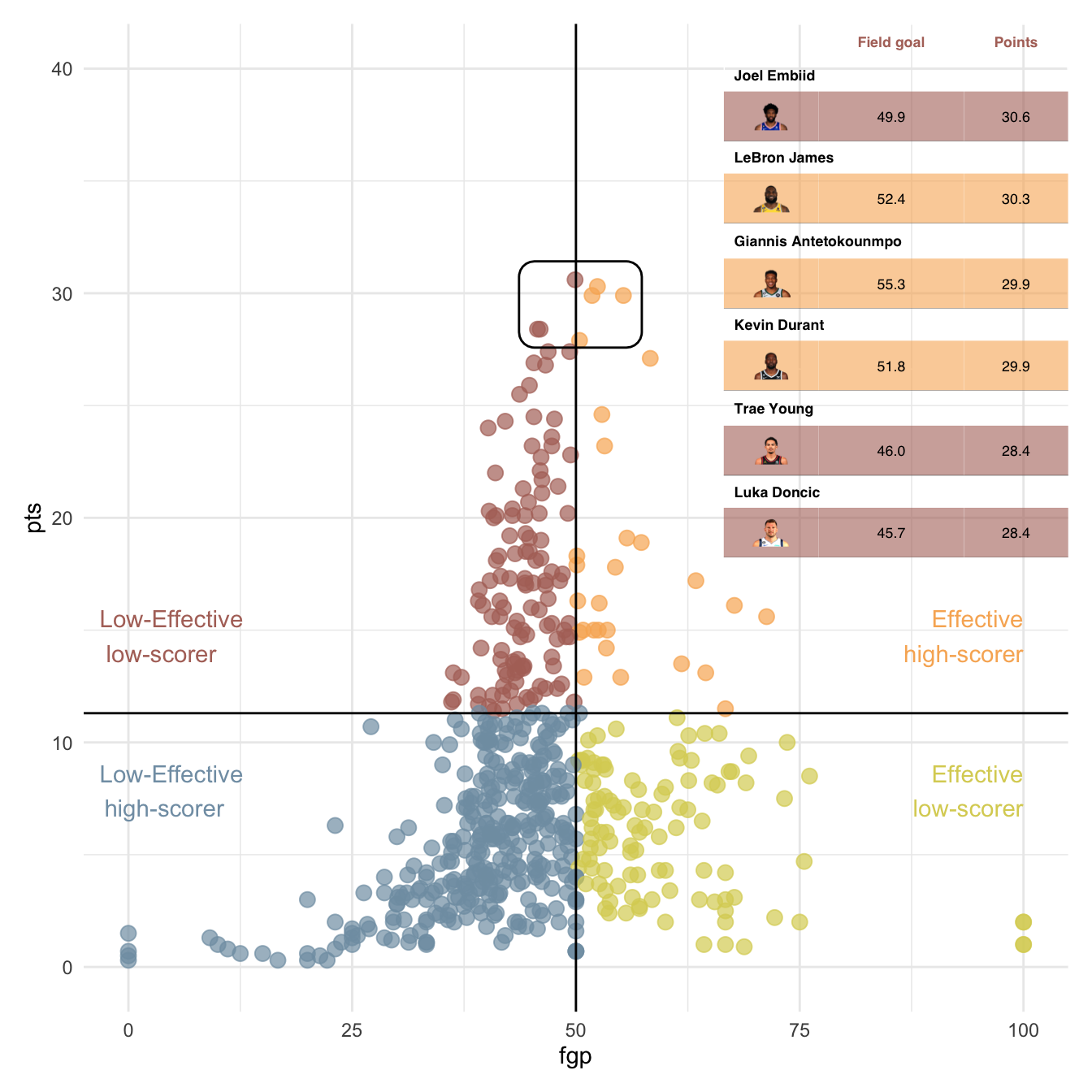
Add flextable inside ggplot
library(patchwork)
gg + inset_element(
    gen_grob(ft, fit = "width"),
    left = 0.65, bottom = .65,
    right = 1, top = 1
  )  + theme(
    plot.background = element_rect(fill = "transparent"),
    panel.background = element_rect(fill = "transparent")
  )
Add flextable next to a ggplot
gg + gen_grob(ft, fit = "width")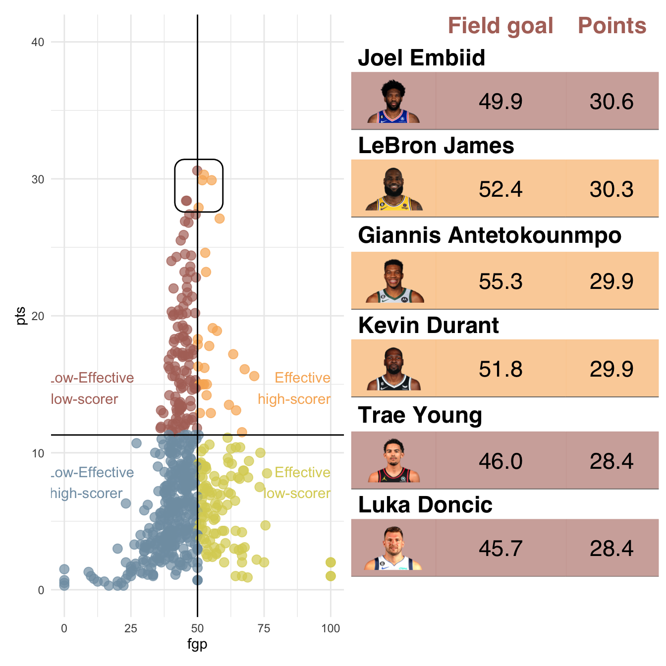
gg + gen_grob(ft, fit = "width") + plot_layout(ncol = 2, widths = c(3, 1))