Shift Tables with flextable

Introduction

Shift tables are tables used in clinical trial analysis.

They show the progression of change from the baseline, with the progression often being along time; the number of subjects is displayed in different range (e.g. low, normal, or high) at baseline and at selected time points or intervals.

The two steps for the creation of these tables are the following:

• Do the calculations, for this we will use function flextable::shift_table(). It calculates the counts and aggregates these counts according to different dimensions in order to display subtotals.
• Create a flextable with function as_flextable().

We used the article by (Luo 2017) to help us understand shift tables.

Sample data

We will illustrate with a dataset named sdtm_lb containing Laboratory Tests Results and available in the “safetyData” package. From the manual of sdtm_lb, it contains:

One record per analyte per planned time point number per time point reference per visit per subject

adlb <- safetyData::sdtm_lb %>% as_tibble() %>% 
  filter(LBTEST %in% c("Albumin", "Alkaline Phosphatase"),
         grepl("(WEEK|SCREENING)", VISIT))
adlb

Calculation of the shift table

The calculation of the shift table is a single call to shift_table():

SHIFT_TABLE <- shift_table(
  x = adlb, cn_visit = "VISIT",
  cn_grade = "LBNRIND",
  cn_usubjid = "USUBJID",
  cn_lab_cat = "LBTEST",
  cn_is_baseline = "LBBLFL",
  baseline_identifier = "Y",
  grade_levels = c("LOW", "NORMAL", "HIGH"))
SHIFT_TABLE

The data.frame produced is containing attributes that you can use for post-treatments, i.e. transform grades and visits as factor columns.

SHIFT_TABLE_VISIT <- attr(SHIFT_TABLE, "VISIT_N")

visit_as_factor <- attr(SHIFT_TABLE, "FUN_VISIT")
range_as_factor <- attr(SHIFT_TABLE, "FUN_GRADE")

# post treatments ----
SHIFT_TABLE <- SHIFT_TABLE |> mutate(
  VISIT = visit_as_factor(VISIT),
  BASELINE = range_as_factor(BASELINE),
  LBNRIND = range_as_factor(LBNRIND))

SHIFT_TABLE_VISIT <- SHIFT_TABLE_VISIT |>
  mutate(VISIT = visit_as_factor(VISIT))

SHIFT_TABLE

In order to have a short table when illustrating, we are going to filter data with only few visits.

SHIFT_TABLE <- SHIFT_TABLE |> 
  filter(VISIT %in% c("WEEK 4", "WEEK 12", "WEEK 16", "WEEK 26"))

Tabulate with tabulator

Now the datasets are ready, we need to define a tabulator object that can then be passed to as_flextable().

my_format <- function(z) {
  formatC(z * 100, digits = 1, format = "f",
          flag = "0", width = 4)
}

tab <- tabulator(
  x = SHIFT_TABLE,
  hidden_data = SHIFT_TABLE_VISIT,
  row_compose = list(
    VISIT = as_paragraph(VISIT, "\n(N=", N_VISIT, ")")
  ),
  rows = c("LBTEST", "VISIT", "BASELINE"),
  columns = c("LBNRIND"),
  `n` = as_paragraph(N),
  `%` = as_paragraph(as_chunk(PCT, formatter = my_format))
)

Production of the flextable

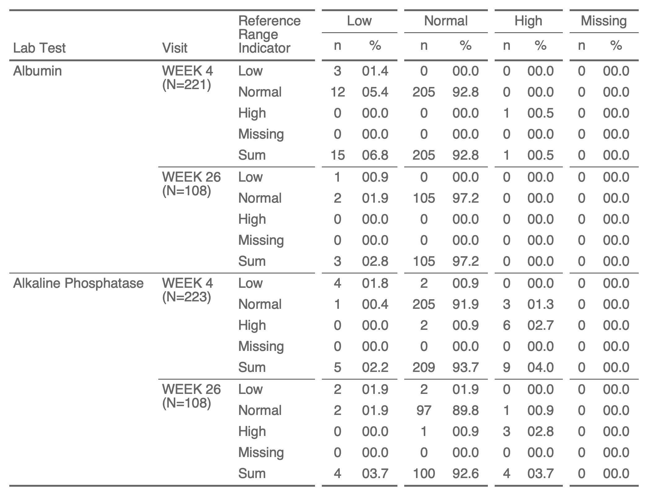
ft <- as_flextable(
  x = tab, separate_with = "VISIT",
  label_rows = c(LBTEST = "Lab Test", VISIT = "Visit",
                 BASELINE = "Reference Range Indicator")) |>
  width(j = 3, width = 0.9)

ft

Word automation

This type of table is often too large to be displayed on a single page of a document. We will use a programmatic approach to generate a Word document containing one sub-table per page with some pagination markers or titles.

First, let’s load package ‘officer’ and define a post processing function that will add the page number (as a Word field) in the top line of the table.

library(officer)

set_flextable_defaults(
  post_process_docx = function(x) {
    x <- add_header_lines(x, "Page N°") |> 
      append_chunks(i = 1, part = "header", j = 1,
                    as_word_field(x = "Page")) |> 
      align(part = "header", align = "right", i = 1) |>
      hline_top(part = "header", border = fp_border_default(width = 0)) 
    x
  }
)

The function that create the flextable for each subset of data is the following:

small_shift_ft <- function(x) {
  tab <- tabulator(
    x = x,
    rows = c("VISIT", "BASELINE"),
    columns = c("LBNRIND"),
    `n` = as_paragraph(N),
    `%` = as_paragraph(as_chunk(PCT, formatter = my_format))
  )
  ft <- as_flextable(
    x = tab, separate_with = "VISIT",
    label_rows = c(VISIT = "Visit", BASELINE = "Reference Range Indicator"))
  ft
}

Then, split or nest sub tables. We will use tidyr::nest().

The Word template being used can be downloaded here: template.docx. We have added our logo and page numbers at the bottom of each page.

subdata <- nest(SHIFT_TABLE, data = all_of(c("VISIT", "BASELINE", "LBNRIND", "N", "PCT")))

doc <- read_docx(path = "template.docx") |> 
  body_add_par("Table of content", style = "Title") |>
  body_add_toc()

for (i in seq_len(nrow(subdata))) {
  
  ft <- small_shift_ft(subdata[[i, "data"]])
  doc <- body_add_break(doc) |>
    body_add_par(subdata[[i, "LBTEST"]], style = "heading 1") |>
    body_add_flextable(ft)

}

print(doc, target = "illustration.docx")

The resulting Word document can be downloaded here: illustration.docx. The miniatures below show the expected document.

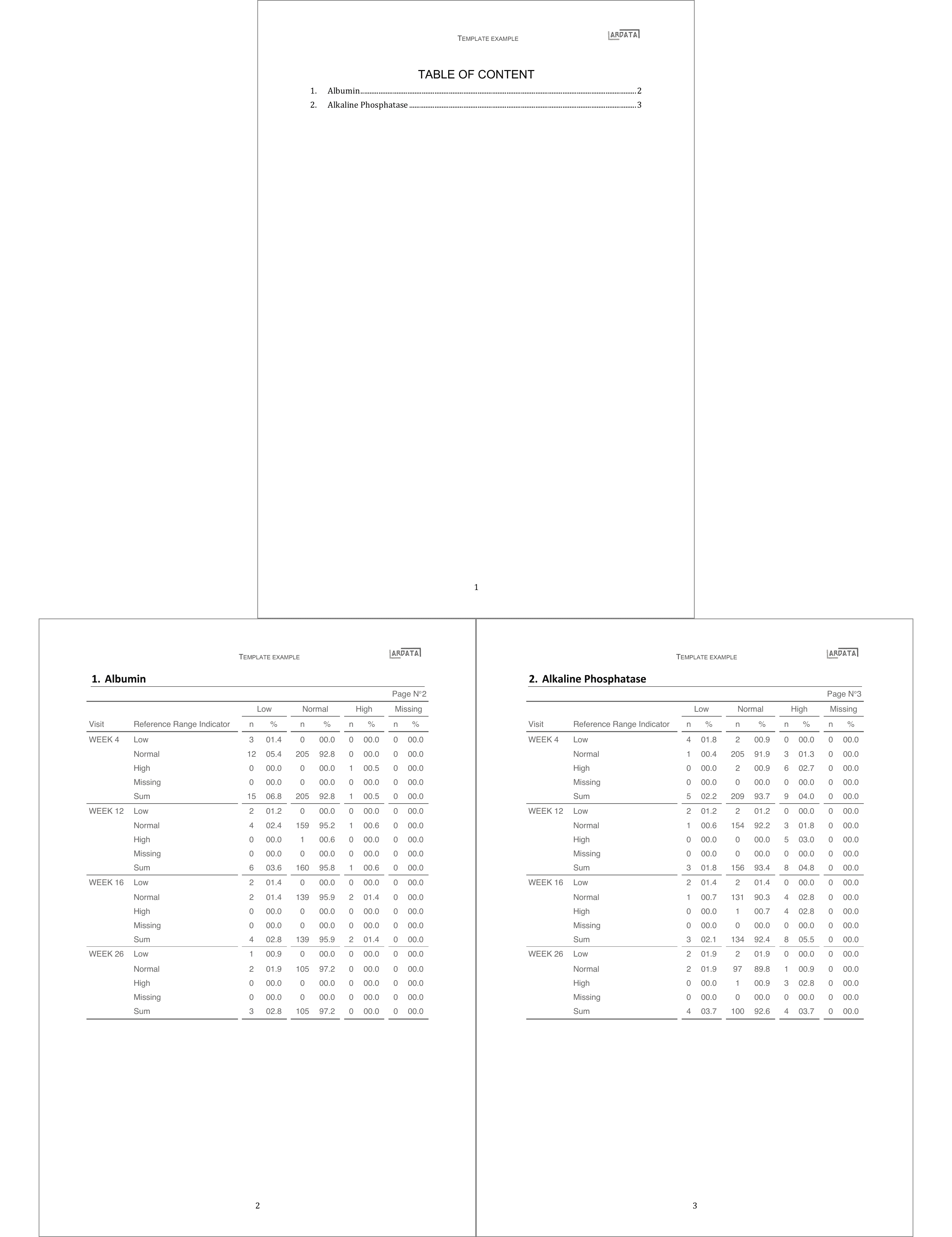
miniatures of resulting Word document