Nice cross-tabulated flextable

Required packages

We will use the following packages:

library(tidyverse)
library(flextable)
library(officer)
use_df_printer()

Sample dataset

The summary of a subset of ggplot2::diamonds will be used to define the content of the flextable.

The code below is filtering some data so that our illustration does not contain too many columns.

dat <- ggplot2::diamonds |>
  filter(
    cut %in% c("Good", "Very Good"),
    clarity %in% c("I1", "SI1", "VS2")
  ) |> 
  mutate(price = price / 1000)
dat

summary_dat <- dat |>
  group_by(cut, color, clarity) |>
  summarise(
    y_mean = mean(price, na.rm = TRUE),
    y_sd = sd(price, na.rm = TRUE),
    .groups = "drop"
  )
summary_dat

cut_counts <- count(dat, cut, name = "n_cut")
cut_counts

clarity_counts <- count(dat, clarity, name = "n_clarity")
clarity_counts

Flextable default settings

This step is not mandatory, it defines some default values for the flextable to be produced later.

# Modify flextable defaults formatting properties ----
init_flextable_defaults()
set_flextable_defaults(
  theme_fun = theme_booktabs,
  big.mark = " ", font.color = "#333333",
  border.color = "#333333",
  padding = 3,
)

Using function tabulator

Now all datasets are ready to be used, let’s call function tabulator() that will prepare an object ready to be sent to as_flextable().

ftd <- fp_text_default(color = "#f24f26")

# create tabulator object to be used with `as_flextable()` ----
tab <- tabulator(
  x = summary_dat,
  rows = c("cut", "color"),
  columns = "clarity",
  hidden_data = cut_counts,
  row_compose = list(
    cut = as_paragraph(cut, as_chunk(x = paste0("\nn = ", n_cut), props = ftd))
  ),
  # defines the only cells to show in the result
  `y stats` = as_paragraph(y_mean, " (\u00B1 ", y_sd, ")")
)


## get colkeys corresponding to multiple "y stats" ----
colkeys <- tabulator_colnames(tab, columns = "y stats")
colkeys
## [1] "I1@y stats"  "SI1@y stats" "VS2@y stats"

The flextable

A flextable is produced with the following code:

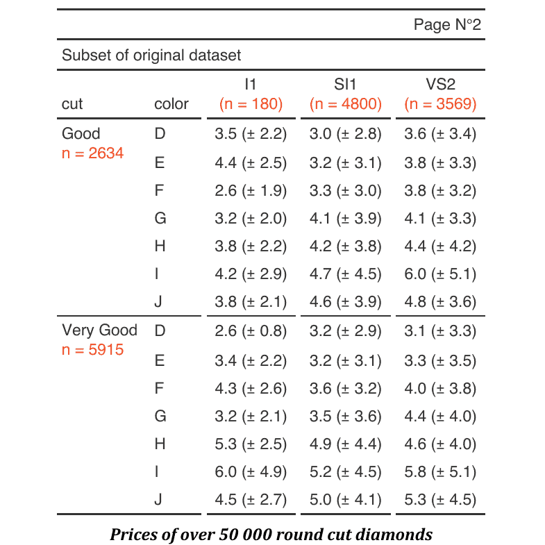
ft <- as_flextable(tab, separate_with = "cut")
ft

Customise the table

We need to add details in the columns headers.

ft <- append_chunks(ft, 
  j = colkeys, i = 1, 
  part = "header",
  as_chunk(fmt_header_n(clarity_counts$n_clarity), props = ftd)
)
ft

Add a title in the header part:

ft <- add_header_lines(ft, "Subset of original dataset")
ft

And add a special line so that when rendered in line the top of the flextable will indicate the page number corresponding to its position in the document.

ft <- add_header_lines(ft, "Page N°") |> 
  append_chunks(i = 1, part = "header", j = 1,
                as_word_field(x = "Page")) |> 
  align(part = "header", align = "right", i = 1) |> 
  set_caption(caption = "Prices of over 50 000 round cut diamonds")

ft

See how it renders in Word

The following code is producing a Word document with package ‘officer’, the content is a fake content. The purpose is to show how the flextable is rendered in a Word document.

psum_txt <- "Lorem ipsum dolor sit amet, purus ut nullam nisl vehicula non ligula sem non. Egestas nascetur, eu sed nec mattis semper arcu auctor sagittis id consequat non? Facilisi vestibulum ac nec primis. Posuere sociis ligula tempor, mattis sed sed dapibus. Taciti nulla mattis aliquet dictumst, nisi aenean, pulvinar! Hendrerit porttitor quis praesent mi nisl lorem mauris ut nulla. Tincidunt in sit sit quisque id molestie. Eros, orci ligula phasellus sed erat vel vivamus penatibus aliquam, scelerisque turpis sociis erat."

landscape_two_columns <- block_section(
  prop_section(
    type = "continuous",
    section_columns = section_columns(widths = c(3, 3))
  )
)

read_docx(path = "template.docx") |> 
  body_add_par(value = "Lorem ipsum", style = "heading 1") |> 
  body_add_par(psum_txt) |> 
  body_add_par(value = "Tempor velit sed", style = "heading 2") |> 
  body_end_block_section(value = block_section(property = prop_section(type = "continuous"))) |> 
  body_add_par(psum_txt) |> 
  body_add_par(psum_txt) |> 
  body_end_block_section(value = landscape_two_columns) |> 
  body_add_par(psum_txt) |> 
  body_add_par(psum_txt) |> 
  body_add_break() |> 
  body_add_par(value = "Mattis potenti metus", style = "heading 2") |> 
  body_add_par(value = "") |> 
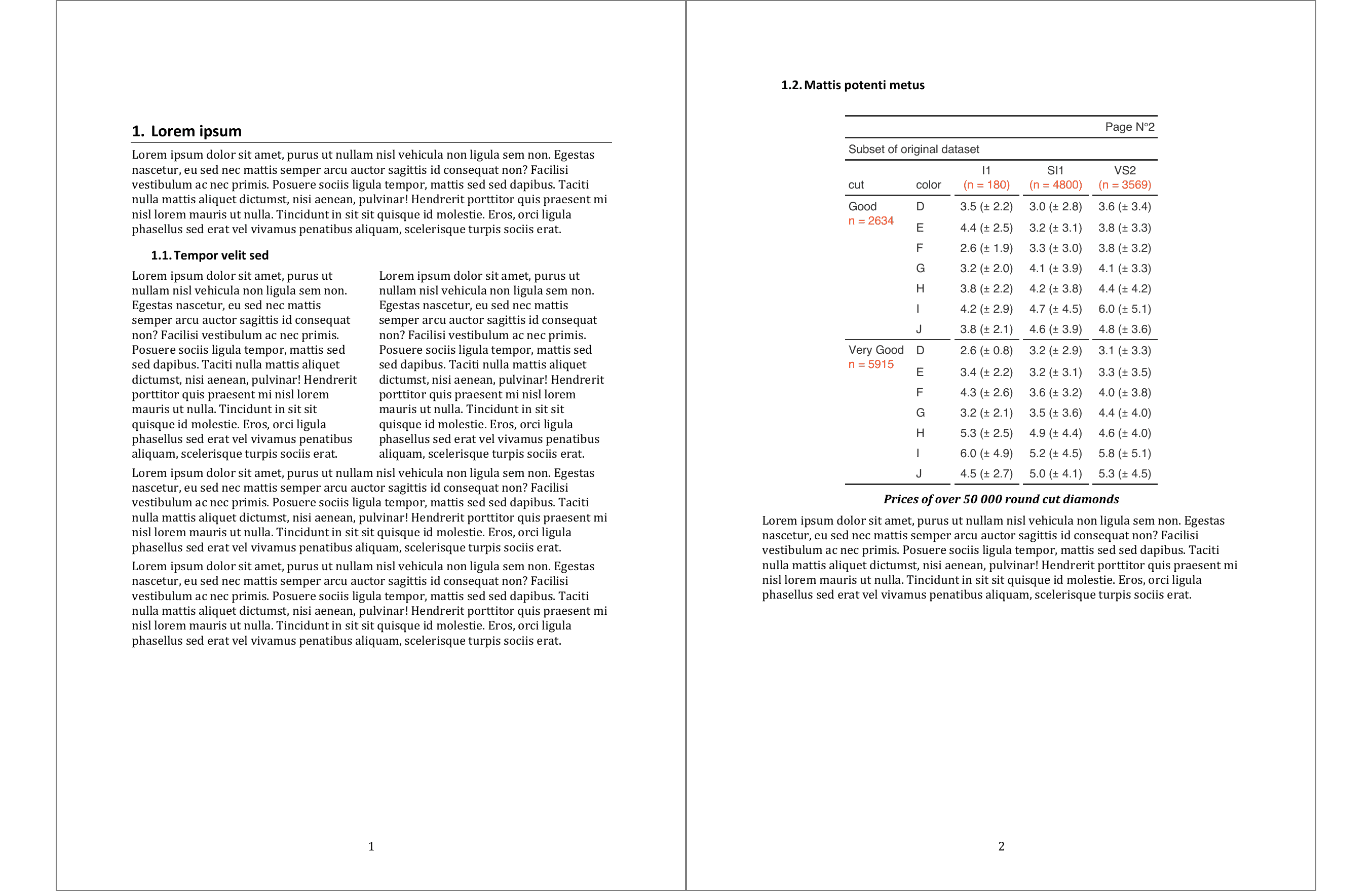
  body_add_flextable(value = ft, topcaption = FALSE, keepnext = FALSE) |> 
  body_add_par(psum_txt) |> 
  print(target = "illustration.docx")

Here is the produced Word document: illustration.docx

After updating the fields in the document, it has this rendering:

illustration