Correlation matrix
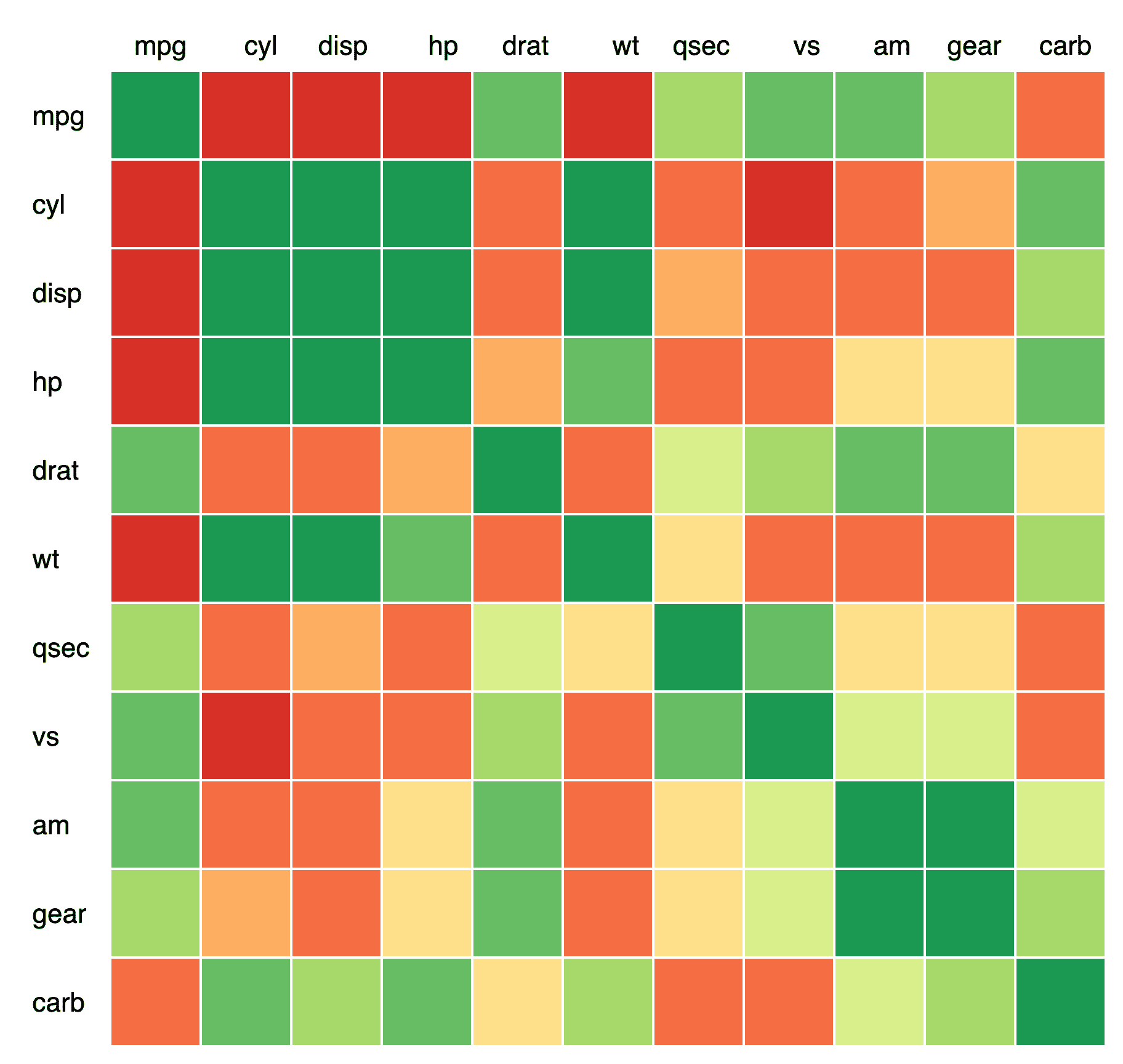
This example uses a correlation matrix as data source. We will first create a data.frame from the correlation matrix and then we will create the reporting table with ‘flextable’.
data
# correlations ----
library(dplyr)
##
## Attachement du package : 'dplyr'
## Les objets suivants sont masqués depuis 'package:stats':
##
##     filter, lag
## Les objets suivants sont masqués depuis 'package:base':
##
##     intersect, setdiff, setequal, union
library(tibble)
correlations <- cor(mtcars) |>
  as.data.frame() |>
  rownames_to_column(var = "rowname")
correlations
##    rowname        mpg        cyl       disp         hp        drat         wt
## 1      mpg  1.0000000 -0.8521620 -0.8475514 -0.7761684  0.68117191 -0.8676594
## 2      cyl -0.8521620  1.0000000  0.9020329  0.8324475 -0.69993811  0.7824958
## 3     disp -0.8475514  0.9020329  1.0000000  0.7909486 -0.71021393  0.8879799
## 4       hp -0.7761684  0.8324475  0.7909486  1.0000000 -0.44875912  0.6587479
## 5     drat  0.6811719 -0.6999381 -0.7102139 -0.4487591  1.00000000 -0.7124406
## 6       wt -0.8676594  0.7824958  0.8879799  0.6587479 -0.71244065  1.0000000
## 7     qsec  0.4186840 -0.5912421 -0.4336979 -0.7082234  0.09120476 -0.1747159
## 8       vs  0.6640389 -0.8108118 -0.7104159 -0.7230967  0.44027846 -0.5549157
## 9       am  0.5998324 -0.5226070 -0.5912270 -0.2432043  0.71271113 -0.6924953
## 10    gear  0.4802848 -0.4926866 -0.5555692 -0.1257043  0.69961013 -0.5832870
## 11    carb -0.5509251  0.5269883  0.3949769  0.7498125 -0.09078980  0.4276059
##           qsec         vs          am       gear        carb
## 1   0.41868403  0.6640389  0.59983243  0.4802848 -0.55092507
## 2  -0.59124207 -0.8108118 -0.52260705 -0.4926866  0.52698829
## 3  -0.43369788 -0.7104159 -0.59122704 -0.5555692  0.39497686
## 4  -0.70822339 -0.7230967 -0.24320426 -0.1257043  0.74981247
## 5   0.09120476  0.4402785  0.71271113  0.6996101 -0.09078980
## 6  -0.17471588 -0.5549157 -0.69249526 -0.5832870  0.42760594
## 7   1.00000000  0.7445354 -0.22986086 -0.2126822 -0.65624923
## 8   0.74453544  1.0000000  0.16834512  0.2060233 -0.56960714
## 9  -0.22986086  0.1683451  1.00000000  0.7940588  0.05753435
## 10 -0.21268223  0.2060233  0.79405876  1.0000000  0.27407284
## 11 -0.65624923 -0.5696071  0.05753435  0.2740728  1.00000000
Background color function
We have to create a function that will allow to associate a background color to the cells according to the value of the corresponding correlation.
We could have done it with the functions available in the ‘scales’ package but we prefer to code the function ourselves to show how to create a coloring function corresponding to a specific need.
The function will associate a color by using cut() function.
cor_color <- function(x){
  col_palette <- c("#D73027", "#F46D43", "#FDAE61", "#FEE08B",
                   "#D9EF8B", "#A6D96A", "#66BD63", "#1A9850")
  mycut <- cut(x,
    breaks = c(-1, -0.75, -0.5, -0.25, 0, 0.25, 0.5, 0.75, 1),
    include.lowest = TRUE, label = FALSE)
  col_palette[mycut]
}

std_border <- fp_border_default(color = "white")
flextable creation
We will apply the cor_color() function to the background colors of
the cells and we will also set a fixed width and height for the cells
in order to reproduce an effect like the heatmap graphics do.
ft <- flextable(correlations) %>%
  border_outer(part = "all", border = std_border) %>%
  border_inner(border = std_border, part = "all") %>%
  compose(i = 1, j = 1, value = as_paragraph(""), part = "header") %>%
  compose(j = ~ . - rowname, value = as_paragraph(""), part = "body") %>%
  bg(j = ~ . - rowname, bg = cor_color) %>%
  height(height = .5) %>%
  hrule(rule = "exact", part = "body") %>%
  width(width = .5)

ftmpg | cyl | disp | hp | drat | wt | qsec | vs | am | gear | carb | |
mpg | |||||||||||
cyl | |||||||||||
disp | |||||||||||
hp | |||||||||||
drat | |||||||||||
wt | |||||||||||
qsec | |||||||||||
vs | |||||||||||
am | |||||||||||
gear | |||||||||||
carb |