Version 0.9 of the ‘flextable’ package adds the possibility to produce tables in RTF documents.
This format is rare but mandatory for some communities, i.e. mainly in the pharmaceutical industry to our knowledge.
Usages
Two methods can be used to embed flextables in an RTF file.
You can use the save_as_rtf() function which produces an RTF file from one or more flextables.
The save_as_rtf() function is a utility function of the `flexable’ package.
The documentation of the function can be found at at this address: https://davidgohel.github.io/flextable/reference/save_as_rtf.html.
If the output is not adapted to your needs, you can use the functions
in the ‘officer’ package dedicated to RTF file production,
i.e. officer::rtf_doc() and officer::rtf_add().
The documentation for rtf_add() can be found at this
address: https://davidgohel.github.io/officer/reference/rtf_add.html.
In the following we will show the use of save_as_rtf() and the result produced.
The table for the illustration
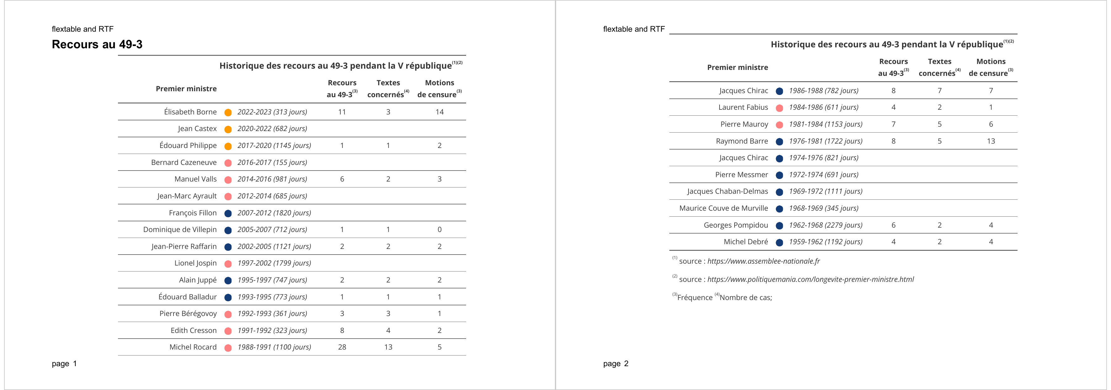
The French news has highlighted some public datasets about the prime ministers of the fifth republic and the uses of the 49-3 article. We have experimented with the data to produce a simple table with flextable.
The data can be downloaded in rds format as well as the script allowing to obtain these data: src-history-49-3.R.
x <- readRDS("history-49-3.RDS")
head(x)
#> couleur name n_nominations debut fin duration
#> 1 CENT Élisabeth Borne 1 2022-05-16 2023-03-25 313
#> 2 CENT Jean Castex 1 2020-07-03 2022-05-16 682
#> 3 CENT Édouard Philippe 2 2017-05-15 2020-07-03 1145
#> 4 GAU Bernard Cazeneuve 1 2016-12-06 2017-05-10 155
#> 5 GAU Manuel Valls 2 2014-03-31 2016-12-06 981
#> 6 GAU Jean-Marc Ayrault 2 2012-05-15 2014-03-31 685
#> n_eng_resp n_text n_censor_motion
#> 1 11 3 14
#> 2 NA NA NA
#> 3 1 1 2
#> 4 NA NA NA
#> 5 6 2 3
#> 6 NA NA NAPreparation
First we declare some general settings for flextable.
set_flextable_defaults(
    font.family = "Open Sans", font.color = "#333333",
    big.mark = "", fmt_date = "%Y", na_str = "",
    theme_fun = theme_vanilla)
The political side of the minister is indicated with a circle whose color is the color generally used in the media. These shapes must be prepared first, the ‘grid’ package is used for this.
library(grid)
library(dplyr)
x$couleur <- mapply(function(z) {
  col <- case_when(
    z %in% "GAU" ~ "#FF8080",
    z %in% "DTE" ~ "#143c77",
    z %in% "CENT" ~ "#ff9900",
    TRUE ~ "transparent"
  )
  circleGrob(gp = gpar(fill = col, col = "transparent"))
}, z = x$couleur, SIMPLIFY = FALSE, USE.NAMES = FALSE)
The flextable
Now we can define the table with the functions of ‘flextable’.
z <- flextable(
  data = x,
  col_keys = c("name", "couleur", "exercice", "n_eng_resp", "n_text", "n_censor_motion")) |>
  mk_par(j = "exercice",
         value = as_paragraph(
           as_i(debut), as_i("-"), as_i(fin),
           as_i(as_bracket(duration, p = " (", s = " jours)")))) |>
  mk_par(j = "couleur", value = as_paragraph(grid_chunk(couleur, width = .15, height = .15))) |>
  align(j = "name", align = "right", part = "all") |>
  align(j = c("n_eng_resp", "n_text", "n_censor_motion"), align = "center", part = "all") |>
  set_header_labels(name = "Premier ministre",
                    period = "Période",
                    couleur = "",
                    n_eng_resp = "Recours\nau 49-3",
                    n_text = "Textes\nconcernés",
                    n_censor_motion = "Motions\nde censure",
                    longeur = "Nombre de jours\nen fonction") |>
  autofit() |>
  width(j = "couleur", width = .3)
z
Premier ministre | Recours | Textes | Motions | ||
|---|---|---|---|---|---|
Élisabeth Borne |
| 2022-2023 (313 jours) | 11 | 3 | 14 |
Jean Castex |
| 2020-2022 (682 jours) | |||
Édouard Philippe |
| 2017-2020 (1145 jours) | 1 | 1 | 2 |
Bernard Cazeneuve |
| 2016-2017 (155 jours) | |||
Manuel Valls |
| 2014-2016 (981 jours) | 6 | 2 | 3 |
Jean-Marc Ayrault |
| 2012-2014 (685 jours) | |||
François Fillon |
| 2007-2012 (1820 jours) | |||
Dominique de Villepin |
| 2005-2007 (712 jours) | 1 | 1 | 0 |
Jean-Pierre Raffarin |
| 2002-2005 (1121 jours) | 2 | 2 | 2 |
Lionel Jospin |
| 1997-2002 (1799 jours) | |||
Alain Juppé |
| 1995-1997 (747 jours) | 2 | 2 | 2 |
Édouard Balladur |
| 1993-1995 (773 jours) | 1 | 1 | 1 |
Pierre Bérégovoy |
| 1992-1993 (361 jours) | 3 | 3 | 1 |
Edith Cresson |
| 1991-1992 (323 jours) | 8 | 4 | 2 |
Michel Rocard |
| 1988-1991 (1100 jours) | 28 | 13 | 5 |
Jacques Chirac |
| 1986-1988 (782 jours) | 8 | 7 | 7 |
Laurent Fabius |
| 1984-1986 (611 jours) | 4 | 2 | 1 |
Pierre Mauroy |
| 1981-1984 (1153 jours) | 7 | 5 | 6 |
Raymond Barre |
| 1976-1981 (1722 jours) | 8 | 5 | 13 |
Jacques Chirac |
| 1974-1976 (821 jours) | |||
Pierre Messmer |
| 1972-1974 (691 jours) | |||
Jacques Chaban-Delmas |
| 1969-1972 (1111 jours) | |||
Maurice Couve de Murville |
| 1968-1969 (345 jours) | |||
Georges Pompidou |
| 1962-1968 (2279 jours) | 6 | 2 | 4 |
Michel Debré |
| 1959-1962 (1192 jours) | 4 | 2 | 4 |


Annotations
It only remains to add some annotations and the table can be sent in an RTF document.
z <- add_header_lines(z,
  values = as_paragraph(
    as_chunk("Historique des recours au 49-3 pendant la V république",
      prop = fp_text_default(font.size = 13, bold = TRUE)
    ))
  ) |>
  footnote(i = 1, j = 1, ref_symbols = "(1)",
           part = "header",
           value = as_paragraph(
             as_chunk(" source : "),
             as_i("https://www.assemblee-nationale.fr")
             )
           ) |>
  footnote(i = 1, j = 1, ref_symbols = "(2)",
           part = "header",
           value = as_paragraph(
             as_chunk(" source : "),
             as_i("https://www.politiquemania.com/longevite-premier-ministre.html")
           )) |>
  footnote(i = 2, j = c(4, 6), ref_symbols = "(3)",
           part = "header",
           value = as_paragraph(
             as_chunk("Fréquence ")
           )) |>
  footnote(i = 2, j = 5, ref_symbols = "(4)", inline = TRUE,
           part = "header",
           value = as_paragraph(
             as_chunk("Nombre de cas")
           )) |>
  hline(i = 1, part = "header", border = fp_border_default(width = 0))
RTF generation
Because the table is quite large, we use a ‘landscape’ orientation; the header and footer are also augmented with some information including automatic page numbering.
These settings are made with the officer::prop_section() function.
library(officer)

sect_properties <- prop_section(
  page_size = page_size(
    width = 8.3, height = 11.7, orient = "landscape"
  ),
  header_default = block_list(fpar("flextable and RTF")),
  footer_default = block_list(fpar("page ", run_word_field(field = "PAGE  \\* MERGEFORMAT"))),
  page_margins = page_mar(bottom = .6, top = .6, right = .5, left = .5)
)
The call to the save_as_rtf() function finally produces the RTF file.
save_as_rtf(
  "Recours au 49-3" = z,
  pr_section = sect_properties,
  path = "49-3.rtf")
The result can be seen below:
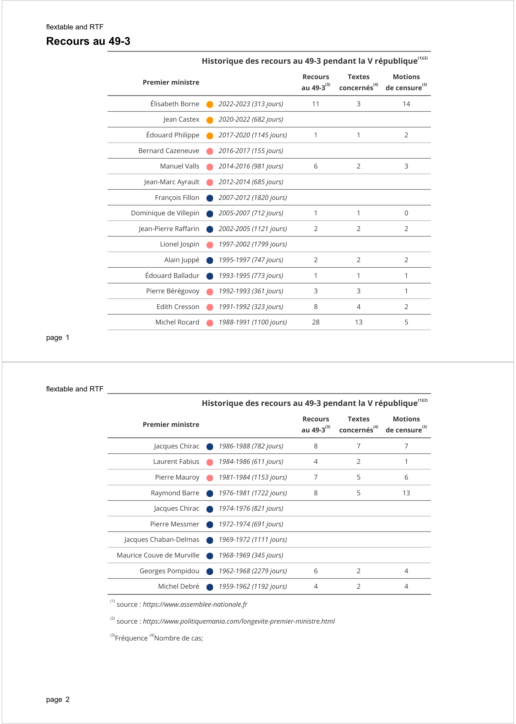
overview of 49-3.rtf